Exploring active learning

I have given a loose introduction to active learning in my previous post.. In this post, I’ll dig deeper into the application of active learning in computer vision.

To understand the problem better, imagine you are asked to prepare a model for classification on a very specific dataset D in which a majority of the samples don’t have labels. This is typically the case in computer vision and NLP application of machine learning where we have to make idiosyncratic models on a dataset that often don’t have labels.

The most common way to solve this problem is to wait for all the images to get labeled and train the models in the conventional supervised-learning way. It requires you to be patient and invest your time and resources in the tedious and humdrum process of data labeling. Data annotation or labeling is, in my humble opinion, a mundane yet key to supervised learning.

The smarter way of dealing with the aforementioned problem is to use active learning. Through active learning, we generate the most promising candidates for model training and get them labeled. Let’s see it in more detail.

Let’s assume that we have a small fraction (Df) of the dataset already labeled. Following are the steps for training models using active learning :

Train a supervised model on the Df
Generate the N most promising candidates Dc from the pool of unlabeled dataset
Integrate the dataset and labels:= Df= Df+Dc
Repeat until a good enough model is trained.

The first step is straight forward; just train the best model you can on the fraction of the dataset that’s labeled. In the next step, we generate predictions on the pool of unlabeled data points. From these predictions, we can find out the subset of predictions in which the model is most uncertain. There are mainly three ways to do this:

Least confidence

It is also referred as uncertainty measurement. Basically, if the model is making a binary classification, the variance between the predicted probabilities tells us about how confident the model is on that sample. In case the model has strong confidence, the probabilities would look like ~ [0.9,0.1] while in the case of low confidence, the probabilities would look like ~ [0.51,0.49].
Margin sampling

This method takes into account the difference between the highest probability and the second-highest probability. As in the above example, the margin in the first case would be 0.9-0.1=0.8 and 0.51-0.49=0.02.
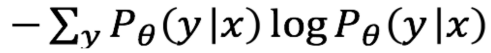
Entropy

The entropy formula is applied to each instance and the instance with the largest value is queried. The formula is shown below-

Lastly, as we get the most promising samples labeled, we integrate it into preexisting labels, and repeat the entire process.

Let’s see it in action. Consider the MNIST dataset. First, we are going to train a supervised model that would utilize the entirety of labels to get a reference performance.

Model definition

def create_keras_model():
    
    model = Sequential()
    model.add(Conv2D(32, kernel_size=(3, 3), activation='relu', input_shape=(28, 28, 1)))
    model.add(Conv2D(64, (3, 3), activation='relu'))
    model.add(MaxPooling2D(pool_size=(2, 2)))
    model.add(Dropout(0.25))
    model.add(Flatten())
    model.add(Dense(128, activation='relu'))
    model.add(Dense(10, activation='softmax'))

    model.compile(loss='categorical_crossentropy', optimizer='adadelta', metrics=['accuracy'])

    return model

Dataset split

from keras.datasets import mnist
from sklearn.model_selection import train_test_split
(X_train, y_train), (X_test, y_test) = mnist.load_data()
X_train = X_train.reshape(60000, 28, 28, 1).astype('float32') / 255
X_test = X_test.reshape(10000, 28, 28, 1).astype('float32') / 255
y_train = keras.utils.to_categorical(y_train, 10)
y_test = keras.utils.to_categorical(y_test, 10)

# for some reason the testset is not a representative of the entire dataset, combining and re-splitting
X = np.concatenate((X_train,X_test),axis=0)
y = np.concatenate((y_train,y_test),axis=0)

X_train, X_test, y_train, y_test = train_test_split(X, y, test_size=0.33, random_state=42)

Notice that I have set apart 33% of the dataset as test-set intened for unbaised evaluation. We will never mix this subset of the dataset with anything.

Supervised training

epochs = 10
model = create_keras_model()
history = model.fit(x=X_train,y=y_train, epochs=epochs, validation_split=0.1,verbose=False)
_,testing_accuracy = model.evaluate(X_test, y_test,verbose=False)

Now that we have a baseline, let’s define the parts of active learning.

Uncertainty Calculation

def uncertain_idx(model,x,new_samples):
    pred = model.predict(x)
    idxs = np.argsort(np.transpose(entropy(np.transpose(pred))))[-new_samples:]
    return idxs,pred

Label Combination

def get_ambigious_labels(model,X_reserve,y_reserve,X_pool,y_pool,new_samples=50):

    idx,pred = uncertain_idx(model, X_reserve,new_samples)

    X_new_points = X_reserve[idx]
    y_new_points = y_reserve[idx]
    
    X_pool = np.concatenate((X_pool,X_new_points),axis=0)
    y_pool = np.concatenate((y_pool,y_new_points),axis=0)
    
    X_reserve = np.delete(X_reserve,idx,axis=0)
    y_reserve = np.delete(y_reserve,idx,axis=0)
    
    return X_reserve,y_reserve,X_pool,y_pool

Fitting helper

def model_fit(X_pool,y_pool):
    model = create_keras_model()
    hist = model.fit(X_pool,y_pool,epochs=epochs,validation_split=0.15,verbose=False)
    return model,hist

Model training using Active Learning

Now, let’s assume that we have only a fraction of dataset labeled. Everytime we train a model, we will generate labels for the samples onto which the model is uncertain. Since in this particular case, the data is already a labeled and we are simulating the environment of active learning, we’ll just get the labels and integrate it to the initial training dataset.

X_pool, X_reserve, y_pool, y_reserve = train_test_split(X_train, y_train, test_size = 0.5)

best_test_acc = 0
for i in tqdm_notebook(range(200)):
    model, hist = model_fit(X_pool, y_pool)

    _,testing_accuracy = model.evaluate(X_test, y_test,verbose=False)

    if best_test_acc < testing_accuracy:
        best_test_acc = testing_accuracy
        print("iteration: {}\t total samples: {}\t training accuracy: {}\t validation accuracy: {}\t testing accuracy: {}".format(i, y_pool.shape[0],round(hist.history["accuracy"][-1],3),
        round(hist.history['val_accuracy'][-1],3),round(testing_accuracy,3)))
    X_reserve,y_reserve,X_pool,y_pool = get_ambigious_labels(model, X_reserve, y_reserve, X_pool, y_pool,new_samples=50)

Observations:

During supervised learning, we used 42210 samples to achieve 88.1 % accuracy on our test-set.
Even in the initial phase, we achieved an 82.4% accuracy with just 18960 samples using active learning.
Later, with 30360 samples, we achieved 87.4% test-accuracy with active learning.

The above experiment validates the efficacy of active learning. It is a semi-supervised way of learning that requires a lesser amount of dataset as compared to supervised learning. You can find my work at kaggle.

Least confidence

Margin sampling

Entropy