Usually, when we train a model on a classification task, we are making the model learn the distinction between classes inadvertently. However, we end up optimizing for learning global features that are useful for a high-level understanding. These models would typically fail to generalize for tasks for which they are not intended. For example, a model for a classification task wouldn’t be able to perform well on a segmentation task. You’d think it’d be easy to classify cars based on the shape and size of the tires(because humans can). But the tires of many cars are often similar and the vision algorithm would struggle if it had only that as a feature. The context or in this case the semantics matter. Hence for distinctiveness, all features i.e. local as well as global features have to contextualize to get a better representation of the class.
Contrastive learning is an approach to learn similarity of representation from data points that are organized in pairs of similar/dissimilar examples. The idea is to train ML models for the classification of similar and dissimilar image pairs. There are 3 main components to contrastive learning:
- Dataset - Samples of similar and dissimilar pairs.
- Representation - A mechanism to get a good representations from images for comparison.
- Similarity Metric - Measurement of similarity or distinctiveness.
SimCLR presents a new framework for learning visual distinction using contrastive learning. In terms of the contrastive learning components mentioned above, SimCLR stands as follows:
Dataset
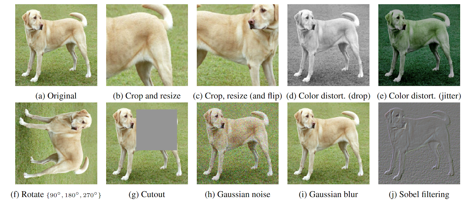
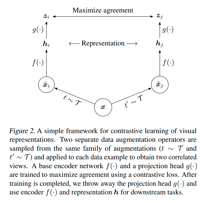
The paper uses an augmentation module that transforms any given image into two correlated samples. The augmentation is relatively straightforward - random cropping that’s followed by resizing to the original dimensions, color distortions, and Gaussian blur. For a minibatch of N examples, image augmentation results in 2N data points. For a given positive pair, the remaining 2(N-1) works as negative samples.

Representation and feature processing
The author used ResNet-50 as an encoder to get the representations in the form of a 2048-D vector. The last average pooling layer gives us this vector. So the pair of images would produce two 2048-D vectors that would then be post-processed using a Projection Head. The projection head is nothing but an MLP with one hidden layer with ReLU whose main function is to map the 2048-D vector to a 128-D vector to a latent space. While we train the MLP with contrastive learning o, it can be used for classification task with very little modification.

Metric
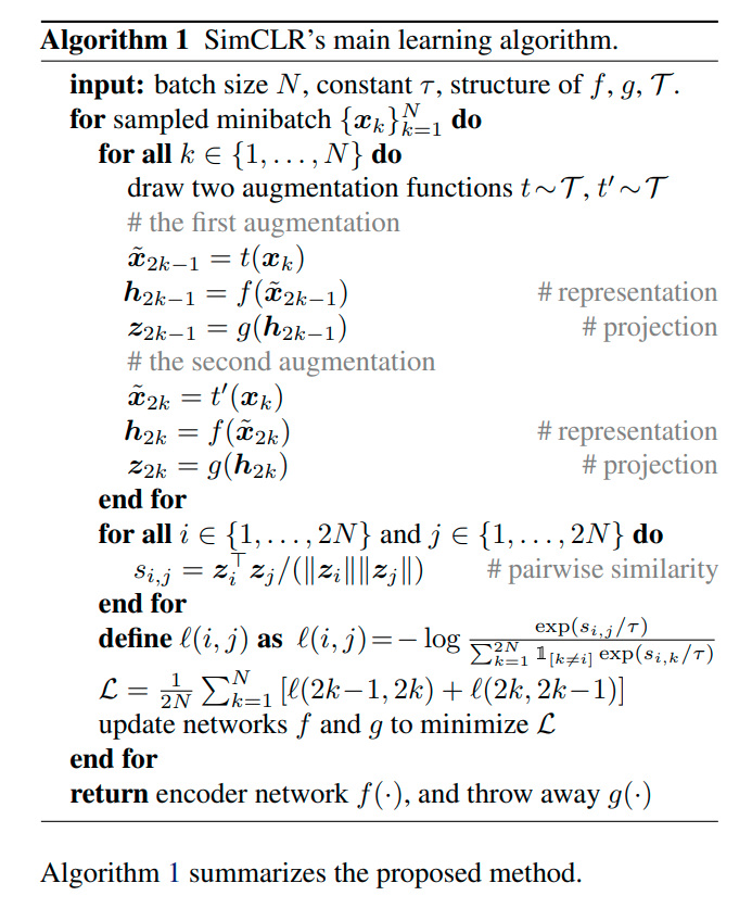
The paper uses a new contrastive loss function in order to measure the distinctiveness(or similarity). From a set of examples that contains a positive pair(zi,zj), the task is to identify zj from the set for a given zi. The metric used to measure the similarity is basically cosine similarity(dot product). Using the similarity we can define the loss function as follow:
 where:
-
sim(zi,zj) = ziTzj / ($\|$ zi$\|$ $\|$zj$\|$)
-
τ = Temperature parameter
The loss is called Normalized temperature-scaled cross-entropy loss.
SimCLR’s proposed algorithm

As you can see, the algorithm is quite simple. The framework is a semi-supervised way of training a discriminator. Here’s an overview:

Batch size and Batch Normalization
A larger batch size provides more negative examples which help in quicker convergence. The author used batch sizes from 256 to 8192. Since ADAM isn’t a great choice for an optimizer after a certain batch size, the authors used the LARS(Layerwise Adaptive Rate Scaling ) optimizer. Also, in distributed training with data parallelism, the computation of positive pairs on the same device can lead to a phenomenon called local information leakage. To tackle this, the authors aggregate the mean and variance for BN overall all devices during training.
Results


Additional observation:
- Composite Augmentation: The authors state that no single augmentation was sufficient but random cropping and random color distortion works very well.
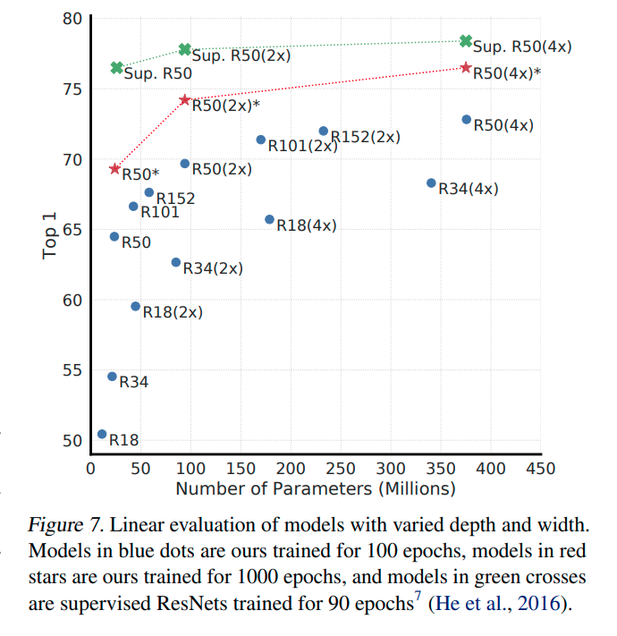
- Unsupervised contrastive learning and bigger model: The difference between the performance of supervised and unsupervised learning shrinks with the bigger models(higher capacity).
- l2 Normalization: Without l2 norm seems necessary for this setup to learn a good representation.
Conclusion
The main contribution of this paper is the contrastive loss function which they named terribly. Of course, as always I am a bit salty about the magnitude of resources used i.e. 128 TPU v3 cores, training a ResNet-50 with a batch size of 4096 for 100 epochs. It’s 2021 and such resources are only available at the top universities and labs. I guess that’s what makes these places so desirable. Having said that, the inference time is actually good since ResNet-50 works like a charm in terms of inference latency. In my experiments, I was getting somewhere from 19 to 25 inferences per second on 1080Ti using an unoptimized clone of this paper.