Introduction to Image Segmentation - II

We looked at the process of image segmentation and its different types in my previous blog. In this post, we are going to take a deeper look at the architecture of U-Net. We will also discuss the PyTorch-based code for U-Net. The complete code can be found at github.

U-Net

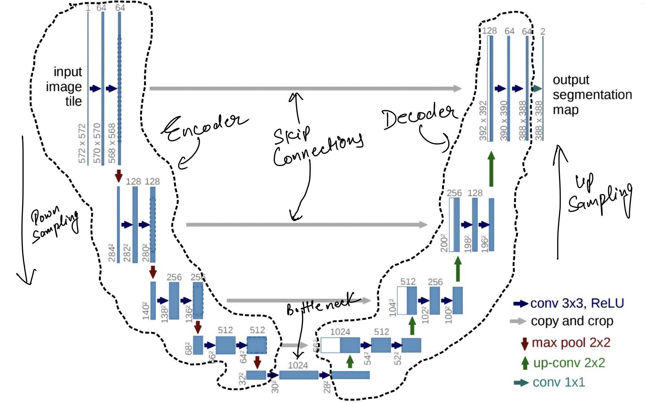
U-Nets are probably the most famous semantic segmentation model. The architecture was primarily developed for biomedical image segmentation however that didn’t stop the community to train it for the semantic segmentation of other objects. The model gets its name from the shape of the architecture as shown in the picture below. The best thing about the model is the amount of data it requires to produce meaningful segmentation maps. I have trained several UNet models that generalize with as little as 80 images. This is great because annotation for semantic segmentation (as well as for instance segmentation) is quite expensive.

Architecture

The model consists of basically 3 parts: a) Encoder b) Decoder c) Bottleneck

The task of the encoder is to learn the features that set the context of the images. This context is finally condensed in the bottleneck. The job of the decoder network is to reconstruct the image using the features from the bottleneck and the various layers of the encoder.

If this sounds gibberish, here’s an oversimplified version. We create a CNN model that downsamples an image from NxNx3 dimension to MxMxno_of_feature. What we have done here is essentially creating a lower-dimensional encoding of the images. This model is called the encoder. Every CNN model that is used from image classification can act as an encoder. For eg, remove the last layer of a ResNet50 and there you go, you have an encoder now.

The decoder network is the opposite of the encoder network. If the encoder downsamples the image to a lower-dimensional encoding, the decoder flips this, i.e., to take an encoding and create a higher dimensional representation which can be a version of the image itself.

Okay, back to the U-Net architecture. So we have an encoder and a decoder. Depending on where you read about the U-Net, some people will also include a bottleneck. The bottleneck is the final layer where we have all the features in the final form. In U-Net, it is used as a sort of intermediate between the encoder and decoder. However, if you want, you can use the encoder+bottleneck configuration and probably train an object classifier by attaching a softmax layer on top of them.

An important feature of the U-Net architecture is the skip connection. I don’t think the original authors called it “skip connection” but it similar to the skip connection found in modern architectures like ResNet. This connection between layers solves a very crucial problem. If you were training a Neural Network in 2014, as you’d increase the depth of the model, you’d face the problem of vanishing gradient. The entire problem of vanishing gradient arises from the fact that backpropagation uses chain rule to update the weight while training and as the depth of a model increases, the gradient to the initial layers gets smaller and smaller. Skip connection helps by skipping few layers and connecting layers that may have multiple blocks of layer in-between. A brilliant explanation can be found here.

Let’s have a look at the code.

The first thing to take a look at is the double convolution unit that’s the part of the encoder as well as the decoder. It has got two convolution layers followed by pooling. The authors didn’t use the batch normalization since their work preceded the batch normalization paper, but we are going to use it. Also, I’m using ReLU6 instead of ReLU as an activation function.

class ConsecutiveConvolution(nn.Module):
    def __init__(self,input_channel,out_channel):
        super(ConsecutiveConvolution,self).__init__()
        self.conv = nn.Sequential(

            nn.Conv2d(input_channel,out_channel,3,1,1,bias=False),
            nn.BatchNorm2d(out_channel),
            nn.ReLU6(inplace=True),
            
            nn.Conv2d(out_channel,out_channel,3,1,1,bias=False),
            nn.BatchNorm2d(out_channel),
            nn.ReLU6(inplace=True),)
        
    def forward(self,x):
        return self.conv(x)

Having defined the consecutive convolution, let’s create the encoder and decoder. The parts of the model are created as soon as the constructor is called.

In the first for loop, we create the encoder by stacking the 4 blocks containing 2 convolution layers back to back. For each block, we use the same number of features mentioned in the paper. The pooling layers would be added during the forward function of the class.

class UNet(nn.Module):
    def __init__(self,input_channel, output_channel, features = [64,128,256,512]):
        super(UNet,self).__init__()
        self.pool = nn.MaxPool2d(kernel_size=2,stride=2)
        self.encoder = nn.ModuleList()
        self.decoder = nn.ModuleList()

        # initialize the encoder
        for feat in features:
            self.encoder.append(
                ConsecutiveConvolution(input_channel, feat)    
            )
            input_channel = feat
        
        #initialize the decoder 
        for feat in reversed(features):
            # the authors used transpose convolution
            self.decoder.append(nn.ConvTranspose2d(feat*2, feat, kernel_size=2, stride=2))
            self.decoder.append(ConsecutiveConvolution(feat*2, feat))
        
        #bottleneck
        self.bottleneck = ConsecutiveConvolution(features[-1],features[-1]*2)
        
        #output layer
        self.final_layer = nn.Conv2d(features[0],output_channel,kernel_size=1)

For the decoder, take a look at the second for loop. We reversed the feature map as the decoder is upsampling(as discussed above). To upsample, the nn.ConvTranspose function of PyTorch is used. Then the next layer would take the input from this layer and the skip connection. This the reason why the output of the first layer is half of the input while the input of the next layer is the same as the input of the first layer. Similar to the encoder, the decoder will contain 4 blocks, each block containing 2 consecutive convolution layers.

We do define our bottleneck there as well along with the final layer that takes the output from the final decoder block and turns it into the shape of an image after convolution.

Okay, so we have the barebones of our model ready. Now we will connect the final components in the forward function.

In the first for loop, we pass the input through the encoder. We also append the gradients from the layers into a list called skip_connection. After that, we apply the pooling layers to further downsample the data. We connect the encoder and the decoder using the bottleneck.

    def forward(self,x):
        skip_connections = []
        
        #encoding
        for layers in self.encoder:
            x = layers(x)
            #skip connection to be used in recreation 
            skip_connections.append(x)
            x = self.pool(x)
        x = self.bottleneck(x)
        
        skip_connections = skip_connections[::-1]
        
        for idx in range(0,len(self.decoder),2):
            x = self.decoder[idx](x)
            skip_connection = skip_connections[idx//2]
            if x.shape != skip_connection.shape[2:]:
                x = TF.resize(x,size=skip_connection.shape[2:])
            concat_skip = torch.cat((skip_connection,x),dim=1)
            x = self.decoder[idx+1](concat_skip)
        
        return self.final_layer(x)

The second for loop shows the data flow for the decoder. We pass the output of the bottleneck output to the first layer of the first block of the decoder. We use the output from the first layer of the decoder block, concate it with the corresponding output in the skip connection and pass it to the second layer in the block. We do this for each block of the decoder. The final output of the decoder is passed through the final layer that recreates a version of the image. It could be the image itself or the mask of the image. In the latter case, it would be performing a semantic segmentation.

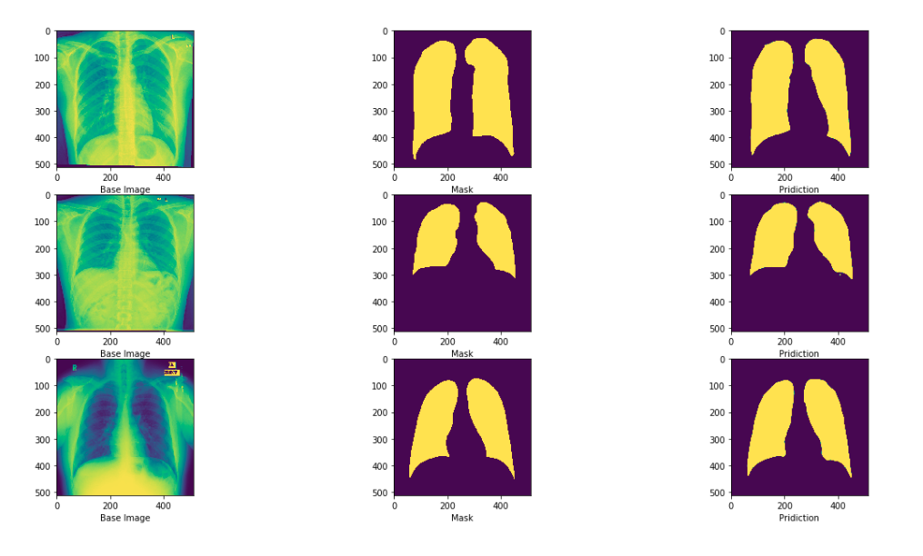
The performace of U-Net can be seen in the image below.

Checkout the source for a keras implementation of U-Net

Training a U-Net

U-Net is trained using Intersection-over-union loss or dice loss. We calculate the dice score/loss using the output mask and the annotated mask. I have used nn.BCEWithLogitsLoss() as the loss function and used adam optimizer. You can have a look at the training file here.

One thing to note is that we have only specified input and output channels. This is because due to the presence of the skip connection, the model becomes symmetric. You can have an input shape as hxwx3 as long as h=w and h%8 = 0.

Conclusion

If you followed along and understood the basic idea behind the U-Net, you have mastered one of the most important tasks of computer vision. If you want to experiment, use different encoders like ResNet, change the decoder model, or change the number of the output channels. The more you toy with the code, the better you get at it.