Should you annotate your data?
As an engineer whose work concerns learning-based architecture in the field of robotics and automation, data generation is one of the easier challenges to overcome. But it is one thing to generate data in heaps and piles and a completely different thing to get a workable machine learning model out of it.
Now, if you choose to develop your models using supervised learning, you’ll have to face the daunting task of completely annotating the data. Data annotation or data labeling is one of the primary consumers of capital, energy, and most importantly, time. Hence, supervised learning is the last thing I consider while designing a solution as the CTO of a startup in the times of COVID.
So what are the alternatives? The answer to this question includes semi-supervised, self-learning, and meta-learning. In this blog, we will look at the technique called Task Agnostic Unsupervised Pretraining.
Task Agnostic Unsupervised Pretraining
Let’s deconstruct the terms used above. When we want to train a deep neural network, the first thing that we do is to create architecture. Once we have defined our layers, hyperparameters, and activation function, we initialize the neural network weights and start the training epochs. As opposed to the random/smart weight initialization, Pretraining aims to set the weights optimally to give the network a headstart. What it means that the model utilizes the dataset with/without labels to learn the relevant features. Think about pretraining as an act of obtaining optimal weights at the network initialization so that the model converges in fewer epochs.
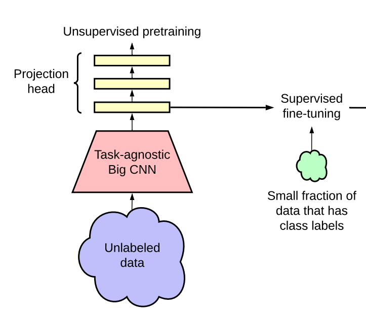
Task agnostic indicates that the pretraining will not be affected by the nature of the task at the hand. Furthermore, all we want to do by pretraining is to learn the relevant features. You can use the features to create any downstream task like object detection, segmentation, etc. Hence, the final use of the pretrained model can be anything that you like but the process of pretraining will remain the same for all of them.
The fact that we need to know right now is that we will be doing all this in an unsupervised fashion. Technically, the pretraining will be unsupervised and then this pretrained model can leverage few samples of supervised data for finetuning. The subsequent finetuning requires as little as 5% of labeled data than the data requirement of a fully supervised model with the same architecture and preformance. Remarkably, the performance of unsupervised pretraining coupled with supervised finetuning on this tiny labeled subset of data is similar and at times even better than training the model using supervised training, employing far more labeled samples.
Technical Details
A sample repository with complete TAUP implementation can be located here at github.
While it would be a tedious task to go into too many details, I’ll try to explain in an abstract manner keeping our focus on main idea.
Model
Okay, here’s the trick. You use a base learner like ResNet, remove the last fully connected layer (as done in transfer learning), and fit a projection head over this decapitated model by adding a couple of fully connected layers. This process resemebles transfer learning to an extent.
class ProjectionHead(nn.Module):
        def __init__(self,in_shape,out_shape=256):
            super().__init__()
            hidden_shape = in_shape//2

            self.layer_1 = nn.Sequential(
                nn.Linear(in_shape,hidden_shape),
                nn.ReLU(inplace=True)
            )

            self.layer_2 = nn.Sequential(
                nn.Linear(hidden_shape,hidden_shape),
                nn.ReLU(inplace=True)
            )

            self.layer_3 = nn.Linear(hidden_shape,out_shape)

        def forward(self,x):
            x = self.layer_1(x)
            x = self.layer_2(x)
            x = self.layer_3(x)

            return x

class ContrastiveModel(nn.Module):
    def __init__(self,backbone):
        super().__init__()
        self.output_dim = 256

        self.backbone=backbone
        self.projectionhead= ProjectionHead(backbone.output_dim)

        self.encoder = nn.Sequential(
                        self.backbone,
                        self.projectionhead,
                        )

    def forward(self,x):
        z   = self.encoder(x)
        return z
The model would take the input and would return a 256 dimension vector. After training this model contrastively ( see here.), we will remove the projection head and add a linear layer for classification.
Dataset
You can use any dataset as long as you have few labeled samples for the supervised fine-tuning part. The best thing about this approach is that you can use as much data as you can possibly produce because the training is unsupervised. As for data augmentation, random-crop, random-horizontal flip, and color jitter should be used. In my testing, these three augmentation techniques yielded a better result than any other combination.
Algorithm
The algorithm to train a TAUP model can be broken down into two board parts as I alluded to earlier. Some of the prominent papers from this domain are simCLR, BYOL, SimSiam, etc. They more or less follow the same pattern.
- Take an image and create a pair by augmenting it.
- The goal is to train a model that produces a similar representation of positive pairs and dissimilar representation of negative pairs. This type of training approach is called Contrastive Learning. Please have a look on my simCLR blog for more details on it.
Here’s a code block for simCLR contrastive learning.
for epoch in global_progress:
    model.train()

    for idx, (image, label) in enumerate(train_loader):
        image = image.to(device)
        aug_image = train_transform(image)
        model.zero_grad()
        z = model.forward(image.to(device, non_blocking=True))
        z_= model.forward(aug_image.to(device,non_blocking=True))
        loss = loss_func(z,z_)
        data_dict['loss'] = loss.item()
        loss.backward()
        optimizer.step()
        scheduler.step()
The last piece of puzzle is the loss function. SimCLR uses NT-Xent loss which is composed of exponentials and cosine similarities.
class ContrastiveLoss(nn.Module):

    def __init__(self, temp=0.5, normalize= False):
        super().__init__()
        self.temp = temp
        self.normalize = normalize

    def forward(self,xi,xj):

        z1 = F.normalize(xi, dim=1)
        z2 = F.normalize(xj, dim=1)

        N, Z = z1.shape
        device = z1.device

        representations = torch.cat([z1, z2], dim=0)
        similarity_matrix = torch.mm(representations, representations.T)

        # create positive matches
        l_pos = torch.diag(similarity_matrix, N)
        r_pos = torch.diag(similarity_matrix, -N)
        positives = torch.cat([l_pos, r_pos]).view(2 * N, 1)

        # print(positives)

        # get the values of every pair that's a mismatch
        diag = torch.eye(2*N, dtype=torch.bool, device=device)
        diag[N:,:N] = diag[:N,N:] = diag[:N,:N]
        negatives = similarity_matrix[~diag].view(2*N, -1)


        logits = torch.cat([positives, negatives], dim=1)
        logits /= self.temp
        labels = torch.zeros(2*N, device=device, dtype=torch.int64)
        loss = F.cross_entropy(logits, labels, reduction='sum')

        return (loss / (2 * N))
This loss function forces (trains) the model to produce a similar representation of positive pairs, i.e, an image and its augmented version. And that’s the crux of the technique. To do this, we use cosine similarity. simCLR and BOYL have a different approach to the use of similarity. simCLR uses positive and negative pairs in the loss function while BOYL just uses positive pairs. Please refer to simCLR implementation and this for a BOYL implementation.
Supervised Fine-tuning
Once we train the base learner with the projection head, we remove the projection head and train a classifier with a linear layer on top of it. This new model requires far fewer labeled examples to converge and that’s the gist of it.
The following code block represents fine-tuning model. The encoder in this model is the ContrastiveModel minus the projection head.
class FineTunedModel(nn.Module):

    def __init__(self, encoder,input_dim, num_classes=10 ):
        super().__init__()
        self.input_dim =  input_dim
        self.num_classes = num_classes
        self.encoder = encoder
        self.fc = nn.Linear(self.input_dim, self.num_classes)
        self.model = nn.Sequential(
                        self.encoder,
                        self.fc
        )

    def forward(self, x):
        z = self.model(x)
        return z
From now on, this pretrained model can be trained in a typical way we train supervised models. The only difference is that this model will converge faster due to the pretraining. And that’s how you reduce the requirement of labelled data samples.
Summary
So, to sum it all up, we leveraged the huge dataset that is usually available to us and trained a base learner using unsupervised contrastive learning. This base learner will learn the representation by using a cosine similarity loss or some different version of it. Once the base learner converges, remove the projection head and replace it with a linear classifier and train your classifier with very few labeled examples and the model converges easily.